Predicting discharge using Bayesian statistics

Our goal is to develop a Bayesian model to predict a patient’s probability of being discharged in the next 24 hours.

Note that, for now in this first attempt, I’m assuming you have some prior knowledge of Bayesian statistics.

Here are three initial steps I think we need to do:

Decide on our “prior” probability and express it as a distribution
Identify some data we can use for the “likelihood”. This can be synthetic to start with
Develop a posterior distribution from the prior and likelihood.

1. Prior probability

We express the probability of discharge as \(\theta\). Our prior belief about \(\theta\) could be that it follows a beta distribution which is expressed as follows:

\[ P(\theta) = Beta(\alpha,\beta) \tag{1}\]

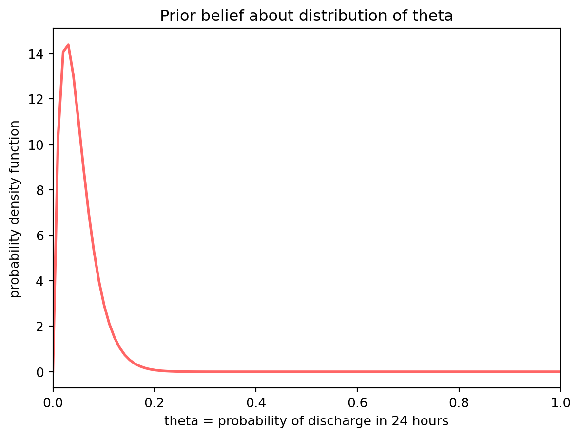
Let’s say we know that 5% of patients are discharged on any given day. Therefore we’d like the expected value of our Beta distribution to be at 0.05. The expected value of a Beta distribution is given by

\[ Exp(\theta) = \frac{\alpha}{\alpha + \beta} \]

If we set \(\alpha\) to be 2 and \(\beta\) to be 38, we’ll get an expected value of 0.05

\[ P(\theta) = Beta(2,38) \tag{2}\]

Plotting this:

Code

import numpy as np
import matplotlib.pyplot as plt
from scipy.stats import beta


a, b = 2, 38
fig, ax = plt.subplots(1, 1)

theta = np.linspace(0, 1, 100)
ax.plot(theta, beta.pdf(theta, a, b),
       'r-', lw=2, alpha=0.6, label='beta pdf')
ax.set_ylabel('probability density function')
ax.set_xlabel('theta = probability of discharge in 24 hours')
ax.set_title('Prior belief about distribution of theta')
plt.xlim([0, 1])

plt.show()

2. Identify some data we can use for the “likelihood”

Now let’s look at some data. This will constitute our likelihood. First let’s read it in from a saved anonymised database

Code

import sqlalchemy as sa
import pandas as pd
import os


sqlite_engine = sa.create_engine('sqlite:///../../data/dummy.db')
df = pd.read_sql_query("SELECT * from discharges", sqlite_engine)
df.head()

# Let N be the number of patients observed
N = df.shape[0]

# Let X be the number of patients who were discharged in 24 hours
X = df[df.hours_to_discharge <= 24].shape[0]
print("Number of people discharged in 24 hours: " + str(X))
print("Total number of people observed: " + str(N))

Number of people discharged in 24 hours: 52
Total number of people observed: 444

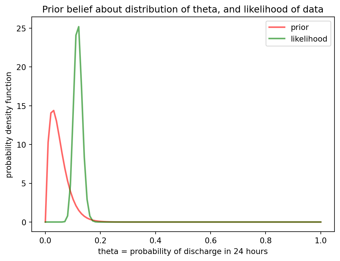
We observe that 52 patients out of 444 were discharged. This provides our likelihood. We can express our data as a binomial distribution where we do N trials with our unknown probability \(\theta\) and return the result we are looking for (ie patient was discharged) X times of the N trials.

\[ P(data) = Binomial(N, \theta) \tag{3}\]

The binomial distribution can be expanded as shown here, where \({N \choose X}\) is the notation for N Choose X (a way of expressing the number of different ways, or permutations, that you could get a result of X discharged patients when starting with N patients in total)

\[ P(data) = {N \choose X} \theta^x(1-\theta)^{(N-X)} \]

We can plot the likelihood

Code

import pandas as pd
import os

#| label: likelihood
#| fig-cap: "Likelihood distribution"

import numpy as np
import matplotlib.pyplot as plt
from scipy.stats import binom
from math import factorial as fact
N_choose_X = fact(N)/(fact(X)*fact(N-X))

fig, ax = plt.subplots(1, 1)


line1, = ax.plot(theta, beta.pdf(theta, a, b),
       'r-', lw=2, alpha=0.6, label='prior')
line2, = ax.plot(theta, N_choose_X*theta**X*(1-theta)**(N-X)*N,
       'g-', lw=2, alpha=0.6, label='likelihood')
ax.legend(handles=[line1, line2])
ax.set_ylabel('probability density function')
ax.set_xlabel('theta = probability of discharge in 24 hours')
ax.set_title('Prior belief about distribution of theta, and likelihood of data')


plt.show()

Now that we have seen the data, we see that our original prior was too pessimistic. A higher proportion of patients are discharged each day than we expected.

3. Develop a posterior distribution from the prior and likelihood

We know from Bayesian statistics that, if you have a beta prior, and binomial likelihood then you can derive the posterior distribution from these without doing any complicated maths.

Specifically, our posterior can be expressed as a beta distribution, in which we can bring in the values of \(\theta\) from our prior, and values of N and X from our likelihood

\[ P(\theta | data) = Beta(\alpha + X,N + \beta - X) \]

And this can also be expressed as

\[ P(\theta | data) = \frac{\theta^{(\alpha + X -1)}(1 - \theta)^{N + \beta - X -1}}{B (\alpha + X -1, N + \beta - X -1)} \] The denominator above is referred to as a normalising constant. It looks confusing, but the key thing to note that it doesn’t contain any values of \(\theta\), making it simpler to work out than when you have to integrate over all values of \(\theta\).

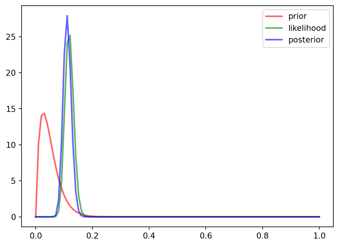
We can now draw our posterior distribution (in blue)

Code

import numpy as np
import matplotlib.pyplot as plt
from scipy.stats import beta


a_prime, b_prime = 2 + X , 38 + N - X
fig, ax = plt.subplots(1, 1)


line1, = ax.plot(theta, beta.pdf(theta, a, b),
       'r-', lw=2, alpha=0.6, label='prior')
line2, = ax.plot(theta, N_choose_X*theta**X*(1-theta)**(N-X)*N,
       'g-', lw=2, alpha=0.6, label='likelihood')
line3, = ax.plot(theta, beta.pdf(theta, a_prime, b_prime),
       'b-', lw=2, alpha=0.6, label='posterior')
ax.legend(handles=[line1, line2, line3])


plt.show()

The posterior predictive distribution is in a tighter range (a taller, slimmer peak) than the prior predictive distribution, and is overwhelmingly determined by the data, rather than the prior. This is the case with Bayesian statistics: as you get more data, the prior beliefs become less important.