from scipy.stats import poisson
lam = 1.4
dist = poisson(lam)
type(dist)scipy.stats._distn_infrastructure.rv_discrete_frozenThe world cup problem
Using the Poisson distribution then the probability of scoring \(k\) goals is
\[ e^{-\lambda}\frac{\lambda^k}{k!} \]
from scipy.stats import poisson
lam = 1.4
dist = poisson(lam)
type(dist)scipy.stats._distn_infrastructure.rv_discrete_frozenThen use the ‘frozen’ random variable above to estimate the probability of a specific value of \(k\). In this context, this is equivalent to estimating the probability of 4 goals from a team that scores on average 1.4 goals per game.
k = 4
dist.pmf(4)0.039471954028253146from empiricaldist import Pmf
import numpy as np
import matplotlib.pyplot as plt
def make_poisson_pmf(lam, qs):
"""
Generate a probability mass function for a Poisson
with mean 'lam' over a range (array) of values 'qs'
"""
ps = poisson(lam).pmf(qs)
pmf = Pmf(ps, qs)
pmf.normalize()
return pmf
lam = 1.4
goals = np.arange(10)
pmf_goals = make_poisson_pmf(lam, goals)
pmf_goals.bar()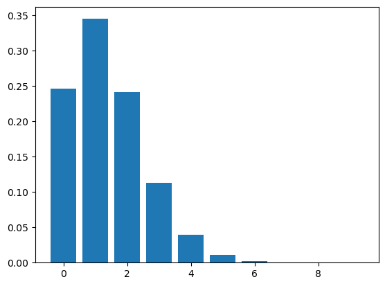
Now being a Bayesian, then we’re really not that interested in the forward problem. We actually want to estimate the goal scoring rate given a number of observed goals: the inverse problem.
So we need to conjecture a set of hypotheses that represents the possible values of \(\lambda\) and then we need to prior that assigns a (prior) probability to each hypothesis.
Here we choose to use the gamma distribution to model the continuous range of possible hypotheses (i.e. a continuous non-negative number). The shape of the gamma is defined by a single parameter \(\alpha\) that represents its mean. And it so happens that the gamma is the conjugate prior of the Poisson.
from scipy.stats import gamma

# mean of gamma is our best guess estimate of goals per game
# given that's the average from previous world cup matches
alpha = 1.4
qs = np.linspace(0,10,101) # hypothesis grid
ps = gamma(alpha).pdf(qs)

prior = Pmf(ps, qs)
prior.normalize()

prior.plot()
<AxesSubplot:>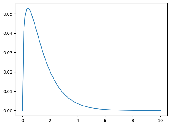
Given an observed number of goals (4) then how does this change our the prior probability distribution over the range of hypotheses.
Here we need to calculate the probabilty of the data (4 goals) for each hypothesis (i.e. the likelihood) which we then multiply by the prior to find the posterior.
# worked example by hand after seeing a team score 4 goals
hypos = np.linspace(0, 10, 101)
likelihood_unnorm = poisson([hypos]).pmf(4)
likelihood = likelihood_unnorm / np.sum(likelihood_unnorm)
plt.plot(likelihood[0]) # <- used [0] b/c array is nested via poisson([])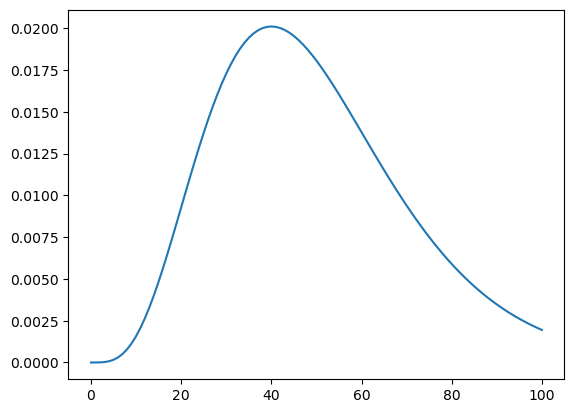
def update_poisson(pmf, data):
    """Update Pmf with a Poisson likelihood"""
    k = data
    lams = pmf.qs # hypotheses over a grid
    likelihood = poisson(lams).pmf(k)
    pmf *= likelihood
    # pmf.normalize() # <- normalize returns a scaler??
    # do this by hand your self
    return pmf / pmf.sum()

# prior
alpha = 1.4
qs = np.linspace(0,10,101) # hypothesis grid
ps = gamma(alpha).pdf(qs)
ps = ps / ps.sum() # normalize


prior = Pmf(ps, qs)

# update (after seeing France score 4 goals)
france = prior.copy()
posterior_f = update_poisson(france, 4)

posterior_f.plot()
plt.plot(prior.qs, prior.ps)
plt.legend(["Posterior", "Prior"])
<matplotlib.legend.Legend at 0x1483ee1f0>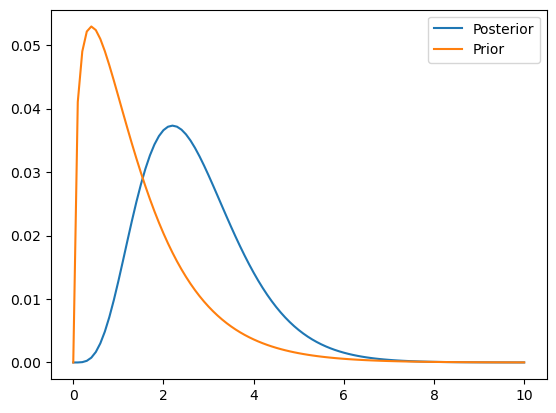
Now repeat the above for Croatia who have scored 2 goals (as opposed to the 4 goals scored by France above)
# update (after seeing Croatia score 2 goals)
croatia = prior.copy()
posterior_c = update_poisson(croatia, 2)

posterior_c.plot()
plt.plot(prior.qs, prior.ps)
plt.legend(["Posterior", "Prior"])
<matplotlib.legend.Legend at 0x148560640>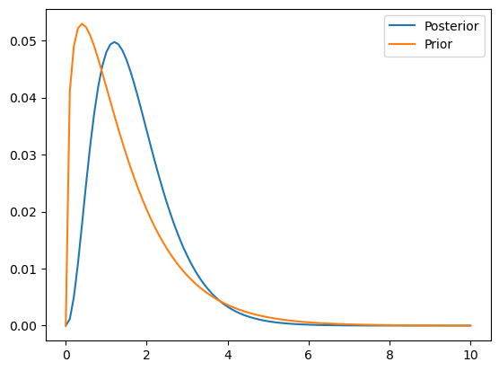
# first sample from the posterior
samples = posterior_f.sample(10**5)
plt.hist(samples, density=True, bins=np.arange(0,10,0.1))
(array([0.00000000e+00, 0.00000000e+00, 1.00002000e-04, 1.40002800e-03,
7.40014800e-03, 1.80003600e-02, 3.04006080e-02, 4.68009360e-02,
7.37014740e-02, 9.94019880e-02, 1.28202564e-01, 1.56103122e-01,
1.92403848e-01, 2.29804596e-01, 2.55605112e-01, 2.78405568e-01,
3.01806036e-01, 3.23906478e-01, 3.25206504e-01, 3.53307066e-01,
3.75207504e-01, 3.64707294e-01, 3.66507330e-01, 3.66107322e-01,
3.75807516e-01, 3.68907378e-01, 3.51807036e-01, 3.36806736e-01,
3.25006500e-01, 3.12506250e-01, 2.92105842e-01, 2.75705514e-01,
2.53905078e-01, 2.54505090e-01, 2.31604632e-01, 2.14604292e-01,
2.02604052e-01, 1.86603732e-01, 1.68603372e-01, 1.53903078e-01,
1.40702814e-01, 1.27302546e-01, 1.18602372e-01, 1.11202224e-01,
1.04102082e-01, 9.05018100e-02, 7.36014720e-02, 7.37014740e-02,
6.56013120e-02, 5.41010820e-02, 4.74009480e-02, 4.64009280e-02,
3.90007800e-02, 3.57007140e-02, 3.47006940e-02, 2.58005160e-02,
2.55005100e-02, 2.15004300e-02, 2.00004000e-02, 1.73003460e-02,
1.57003140e-02, 1.48002960e-02, 1.21002420e-02, 1.16002320e-02,
8.30016600e-03, 6.90013800e-03, 7.40014800e-03, 6.90013800e-03,
6.30012600e-03, 5.20010400e-03, 4.90009800e-03, 4.60009200e-03,
3.70007400e-03, 3.60007200e-03, 2.10004200e-03, 1.90003800e-03,
1.60003200e-03, 1.00002000e-03, 9.00018000e-04, 1.20002400e-03,
9.00018000e-04, 8.00016000e-04, 5.00010000e-04, 1.00002000e-03,
7.00014000e-04, 4.00008000e-04, 4.00008000e-04, 5.00010000e-04,
3.00006000e-04, 5.00010000e-04, 2.00004000e-04, 1.00002000e-04,
0.00000000e+00, 1.00002000e-04, 1.00002000e-04, 0.00000000e+00,
1.00002000e-04, 1.00002000e-04, 4.00008000e-04]),
array([0. , 0.1, 0.2, 0.3, 0.4, 0.5, 0.6, 0.7, 0.8, 0.9, 1. , 1.1, 1.2,
1.3, 1.4, 1.5, 1.6, 1.7, 1.8, 1.9, 2. , 2.1, 2.2, 2.3, 2.4, 2.5,
2.6, 2.7, 2.8, 2.9, 3. , 3.1, 3.2, 3.3, 3.4, 3.5, 3.6, 3.7, 3.8,
3.9, 4. , 4.1, 4.2, 4.3, 4.4, 4.5, 4.6, 4.7, 4.8, 4.9, 5. , 5.1,
5.2, 5.3, 5.4, 5.5, 5.6, 5.7, 5.8, 5.9, 6. , 6.1, 6.2, 6.3, 6.4,
6.5, 6.6, 6.7, 6.8, 6.9, 7. , 7.1, 7.2, 7.3, 7.4, 7.5, 7.6, 7.7,
7.8, 7.9, 8. , 8.1, 8.2, 8.3, 8.4, 8.5, 8.6, 8.7, 8.8, 8.9, 9. ,
9.1, 9.2, 9.3, 9.4, 9.5, 9.6, 9.7, 9.8, 9.9]),
<BarContainer object of 99 artists>)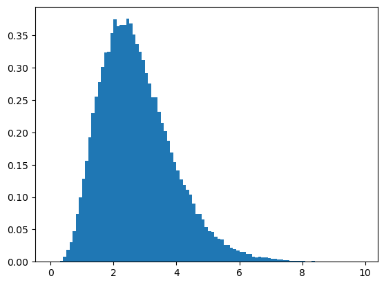
# now for each sample of lambda, you must generate a poisson
# and then you must average those
import pandas as pd
post_pred_dists = pd.DataFrame([make_poisson_pmf(lam, np.arange(10))
for lam in samples[:101] ])post_pred_dists.T| ... | |||||||||||||||||||||||||||||||||||||||||||||||||||||||||||||||||||||||||||||||||
|---|---|---|---|---|---|---|---|---|---|---|---|---|---|---|---|---|---|---|---|---|---|---|---|---|---|---|---|---|---|---|---|---|---|---|---|---|---|---|---|---|---|---|---|---|---|---|---|---|---|---|---|---|---|---|---|---|---|---|---|---|---|---|---|---|---|---|---|---|---|---|---|---|---|---|---|---|---|---|---|---|---|
| 0 | 0.246598 | 0.301194 | 4.493290e-01 | 0.036964 | 0.045112 | 0.002969 | 0.011302 | 0.030298 | 0.301194 | 0.090736 | 0.082108 | 0.100273 | 0.122465 | 0.272532 | 4.065697e-01 | 0.135342 | 0.332871 | 0.122465 | 0.090736 | 0.135342 | 0.165302 | 0.201898 | 0.049842 | 0.074301 | 0.082108 | 0.100273 | 0.090736 | 0.010252 | 0.015164 | 4.065697e-01 | 0.182686 | 0.055070 | 0.110814 | 0.030298 | 0.110814 | 0.005222 | 0.110814 | 0.030298 | 0.149573 | 0.272532 | ... | 0.055070 | 0.074301 | 0.272532 | 0.049842 | 0.022501 | 0.272532 | 0.165302 | 0.036964 | 0.055070 | 0.045112 | 0.036964 | 0.301194 | 0.122465 | 0.122465 | 0.022501 | 0.049842 | 0.182686 | 0.055070 | 0.082108 | 0.165302 | 0.018466 | 0.165302 | 0.055070 | 0.067239 | 0.272532 | 0.100273 | 0.036964 | 0.246598 | 0.006959 | 0.030298 | 0.045112 | 0.082108 | 4.965853e-01 | 0.040834 | 0.040834 | 0.036964 | 0.223131 | 0.033464 | 0.009302 | 0.201898 |
| 1 | 0.345237 | 0.361433 | 3.594632e-01 | 0.121982 | 0.139848 | 0.017515 | 0.050860 | 0.106042 | 0.361433 | 0.217767 | 0.205269 | 0.230629 | 0.257176 | 0.354292 | 3.659127e-01 | 0.270683 | 0.366158 | 0.257176 | 0.217767 | 0.270683 | 0.297544 | 0.323037 | 0.149526 | 0.193184 | 0.205269 | 0.230629 | 0.217767 | 0.047159 | 0.063690 | 3.659127e-01 | 0.310566 | 0.159704 | 0.243792 | 0.106042 | 0.243792 | 0.027675 | 0.243792 | 0.106042 | 0.284189 | 0.354292 | ... | 0.159704 | 0.193184 | 0.354292 | 0.149526 | 0.085505 | 0.354292 | 0.297544 | 0.121982 | 0.159704 | 0.139848 | 0.121982 | 0.361433 | 0.257176 | 0.257176 | 0.085505 | 0.149526 | 0.310566 | 0.159704 | 0.205269 | 0.297544 | 0.073863 | 0.297544 | 0.159704 | 0.181546 | 0.354292 | 0.230629 | 0.121982 | 0.345237 | 0.034797 | 0.106042 | 0.139848 | 0.205269 | 3.476097e-01 | 0.130669 | 0.130669 | 0.121982 | 0.334697 | 0.113777 | 0.043719 | 0.323037 |
| 2 | 0.241666 | 0.216860 | 1.437853e-01 | 0.201271 | 0.216765 | 0.051670 | 0.114435 | 0.185574 | 0.216860 | 0.261320 | 0.256587 | 0.265223 | 0.270035 | 0.230290 | 1.646607e-01 | 0.270683 | 0.201387 | 0.270035 | 0.261320 | 0.270683 | 0.267789 | 0.258429 | 0.224289 | 0.251139 | 0.256587 | 0.265223 | 0.261320 | 0.108466 | 0.133749 | 1.646607e-01 | 0.263981 | 0.231571 | 0.268171 | 0.185574 | 0.268171 | 0.073338 | 0.268171 | 0.185574 | 0.269980 | 0.230290 | ... | 0.231571 | 0.251139 | 0.230290 | 0.224289 | 0.162459 | 0.230290 | 0.267789 | 0.201271 | 0.231571 | 0.216765 | 0.201271 | 0.216860 | 0.270035 | 0.270035 | 0.162459 | 0.224289 | 0.263981 | 0.231571 | 0.256587 | 0.267789 | 0.147726 | 0.267789 | 0.231571 | 0.245087 | 0.230290 | 0.265223 | 0.201271 | 0.241666 | 0.086993 | 0.185574 | 0.216765 | 0.256587 | 1.216634e-01 | 0.209071 | 0.209071 | 0.201271 | 0.251022 | 0.193421 | 0.102739 | 0.258429 |
| 3 | 0.112777 | 0.086744 | 3.834274e-02 | 0.221398 | 0.223991 | 0.101617 | 0.171652 | 0.216503 | 0.086744 | 0.209056 | 0.213822 | 0.203337 | 0.189025 | 0.099792 | 4.939822e-02 | 0.180455 | 0.073842 | 0.189025 | 0.209056 | 0.180455 | 0.160674 | 0.137829 | 0.224289 | 0.217654 | 0.213822 | 0.203337 | 0.209056 | 0.166315 | 0.187249 | 4.939822e-02 | 0.149589 | 0.223852 | 0.196659 | 0.216503 | 0.196659 | 0.129564 | 0.196659 | 0.216503 | 0.170987 | 0.099792 | ... | 0.223852 | 0.217654 | 0.099792 | 0.224289 | 0.205782 | 0.099792 | 0.160674 | 0.221398 | 0.223852 | 0.223991 | 0.221398 | 0.086744 | 0.189025 | 0.189025 | 0.205782 | 0.224289 | 0.149589 | 0.223852 | 0.213822 | 0.160674 | 0.196969 | 0.160674 | 0.223852 | 0.220578 | 0.099792 | 0.203337 | 0.221398 | 0.112777 | 0.144989 | 0.216503 | 0.223991 | 0.213822 | 2.838813e-02 | 0.223009 | 0.223009 | 0.221398 | 0.125511 | 0.219211 | 0.160957 | 0.137829 |
| 4 | 0.039472 | 0.026023 | 7.668548e-03 | 0.182653 | 0.173593 | 0.149885 | 0.193108 | 0.189440 | 0.026023 | 0.125434 | 0.133639 | 0.116919 | 0.099238 | 0.032432 | 1.111460e-02 | 0.090228 | 0.020307 | 0.099238 | 0.125434 | 0.090228 | 0.072303 | 0.055132 | 0.168217 | 0.141475 | 0.133639 | 0.116919 | 0.125434 | 0.191263 | 0.196611 | 1.111460e-02 | 0.063575 | 0.162293 | 0.108162 | 0.189440 | 0.108162 | 0.171672 | 0.108162 | 0.189440 | 0.081219 | 0.032432 | ... | 0.162293 | 0.141475 | 0.032432 | 0.168217 | 0.195492 | 0.032432 | 0.072303 | 0.182653 | 0.162293 | 0.173593 | 0.182653 | 0.026023 | 0.099238 | 0.099238 | 0.195492 | 0.168217 | 0.063575 | 0.162293 | 0.133639 | 0.072303 | 0.196969 | 0.072303 | 0.162293 | 0.148890 | 0.032432 | 0.116919 | 0.182653 | 0.039472 | 0.181236 | 0.189440 | 0.173593 | 0.133639 | 4.967922e-03 | 0.178407 | 0.178407 | 0.182653 | 0.047067 | 0.186329 | 0.189125 | 0.055132 |
| 5 | 0.011052 | 0.006246 | 1.226968e-03 | 0.120551 | 0.107627 | 0.176864 | 0.173798 | 0.132608 | 0.006246 | 0.060208 | 0.066819 | 0.053783 | 0.041680 | 0.008432 | 2.000628e-03 | 0.036091 | 0.004467 | 0.041680 | 0.060208 | 0.036091 | 0.026029 | 0.017642 | 0.100930 | 0.073567 | 0.066819 | 0.053783 | 0.060208 | 0.175962 | 0.165154 | 2.000628e-03 | 0.021616 | 0.094130 | 0.047591 | 0.132608 | 0.047591 | 0.181972 | 0.047591 | 0.132608 | 0.030863 | 0.008432 | ... | 0.094130 | 0.073567 | 0.008432 | 0.100930 | 0.148574 | 0.008432 | 0.026029 | 0.120551 | 0.094130 | 0.107627 | 0.120551 | 0.006246 | 0.041680 | 0.041680 | 0.148574 | 0.100930 | 0.021616 | 0.094130 | 0.066819 | 0.026029 | 0.157575 | 0.026029 | 0.094130 | 0.080401 | 0.008432 | 0.053783 | 0.120551 | 0.011052 | 0.181236 | 0.132608 | 0.107627 | 0.066819 | 6.955091e-04 | 0.114181 | 0.114181 | 0.120551 | 0.014120 | 0.126704 | 0.177777 | 0.017642 |
| 6 | 0.002579 | 0.001249 | 1.635957e-04 | 0.066303 | 0.055608 | 0.173916 | 0.130348 | 0.077355 | 0.001249 | 0.024083 | 0.027841 | 0.020617 | 0.014588 | 0.001827 | 3.000942e-04 | 0.012030 | 0.000819 | 0.014588 | 0.024083 | 0.012030 | 0.007809 | 0.004705 | 0.050465 | 0.031879 | 0.027841 | 0.020617 | 0.024083 | 0.134904 | 0.115607 | 3.000942e-04 | 0.006124 | 0.045496 | 0.017450 | 0.077355 | 0.017450 | 0.160742 | 0.017450 | 0.077355 | 0.009773 | 0.001827 | ... | 0.045496 | 0.031879 | 0.001827 | 0.050465 | 0.094097 | 0.001827 | 0.007809 | 0.066303 | 0.045496 | 0.055608 | 0.066303 | 0.001249 | 0.014588 | 0.014588 | 0.094097 | 0.050465 | 0.006124 | 0.045496 | 0.027841 | 0.007809 | 0.105050 | 0.007809 | 0.045496 | 0.036180 | 0.001827 | 0.020617 | 0.066303 | 0.002579 | 0.151030 | 0.077355 | 0.055608 | 0.027841 | 8.114273e-05 | 0.060896 | 0.060896 | 0.066303 | 0.003530 | 0.071799 | 0.139259 | 0.004705 |
| 7 | 0.000516 | 0.000214 | 1.869665e-05 | 0.031257 | 0.024626 | 0.146587 | 0.083795 | 0.038677 | 0.000214 | 0.008257 | 0.009943 | 0.006774 | 0.004376 | 0.000339 | 3.858353e-05 | 0.003437 | 0.000129 | 0.004376 | 0.008257 | 0.003437 | 0.002008 | 0.001075 | 0.021628 | 0.011841 | 0.009943 | 0.006774 | 0.008257 | 0.088651 | 0.069364 | 3.858353e-05 | 0.001487 | 0.018848 | 0.005484 | 0.038677 | 0.005484 | 0.121705 | 0.005484 | 0.038677 | 0.002653 | 0.000339 | ... | 0.018848 | 0.011841 | 0.000339 | 0.021628 | 0.051081 | 0.000339 | 0.002008 | 0.031257 | 0.018848 | 0.024626 | 0.031257 | 0.000214 | 0.004376 | 0.004376 | 0.051081 | 0.021628 | 0.001487 | 0.018848 | 0.009943 | 0.002008 | 0.060029 | 0.002008 | 0.018848 | 0.013955 | 0.000339 | 0.006774 | 0.031257 | 0.000516 | 0.107878 | 0.038677 | 0.024626 | 0.009943 | 8.114273e-06 | 0.027838 | 0.027838 | 0.031257 | 0.000756 | 0.034874 | 0.093502 | 0.001075 |
| 8 | 0.000090 | 0.000032 | 1.869665e-06 | 0.012894 | 0.009543 | 0.108108 | 0.047135 | 0.016921 | 0.000032 | 0.002477 | 0.003107 | 0.001948 | 0.001149 | 0.000055 | 4.340648e-06 | 0.000859 | 0.000018 | 0.001149 | 0.002477 | 0.000859 | 0.000452 | 0.000215 | 0.008110 | 0.003848 | 0.003107 | 0.001948 | 0.002477 | 0.050974 | 0.036416 | 4.340648e-06 | 0.000316 | 0.006833 | 0.001508 | 0.016921 | 0.001508 | 0.080629 | 0.001508 | 0.016921 | 0.000630 | 0.000055 | ... | 0.006833 | 0.003848 | 0.000055 | 0.008110 | 0.024264 | 0.000055 | 0.000452 | 0.012894 | 0.006833 | 0.009543 | 0.012894 | 0.000032 | 0.001149 | 0.001149 | 0.024264 | 0.008110 | 0.000316 | 0.006833 | 0.003107 | 0.000452 | 0.030014 | 0.000452 | 0.006833 | 0.004710 | 0.000055 | 0.001948 | 0.012894 | 0.000090 | 0.067424 | 0.016921 | 0.009543 | 0.003107 | 7.099989e-07 | 0.011135 | 0.011135 | 0.012894 | 0.000142 | 0.014821 | 0.054933 | 0.000215 |
| 9 | 0.000014 | 0.000004 | 1.661924e-07 | 0.004728 | 0.003287 | 0.070871 | 0.023567 | 0.006581 | 0.000004 | 0.000661 | 0.000863 | 0.000498 | 0.000268 | 0.000008 | 4.340648e-07 | 0.000191 | 0.000002 | 0.000268 | 0.000661 | 0.000191 | 0.000090 | 0.000038 | 0.002703 | 0.001112 | 0.000863 | 0.000498 | 0.000661 | 0.026054 | 0.016994 | 4.340648e-07 | 0.000060 | 0.002202 | 0.000369 | 0.006581 | 0.000369 | 0.047482 | 0.000369 | 0.006581 | 0.000133 | 0.000008 | ... | 0.002202 | 0.001112 | 0.000008 | 0.002703 | 0.010245 | 0.000008 | 0.000090 | 0.004728 | 0.002202 | 0.003287 | 0.004728 | 0.000004 | 0.000268 | 0.000268 | 0.010245 | 0.002703 | 0.000060 | 0.002202 | 0.000863 | 0.000090 | 0.013340 | 0.000090 | 0.002202 | 0.001413 | 0.000008 | 0.000498 | 0.004728 | 0.000014 | 0.037458 | 0.006581 | 0.003287 | 0.000863 | 5.522213e-08 | 0.003959 | 0.003959 | 0.004728 | 0.000024 | 0.005599 | 0.028687 | 0.000038 |
10 rows × 101 columns
(post_pred_dists.T * np.array(france)).sum(axis=1)0 0.006444
1 0.011323
2 0.011493
3 0.008816
4 0.005671
5 0.003244
6 0.001715
7 0.000856
8 0.000408
9 0.000186
dtype: float64